Deep Learning - Generative Adversarial Network

Bhaskar S

05/25/2025

Generative Adversarial Network

Generative Adversarial Network (or GAN for short) is a pair of neural network models that are engaged in an adversarial competition with each other just like a counterfeiter and a cop. One model is referred to as the Generator and the other model is referred to as the Discriminator. The Generator is trying to generate synthetic data samples that are indistiguisable from the real data samples, while the Discriminator is trying to distinguish between the synthetic samples and the real samples.

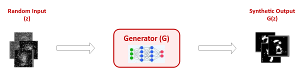
The Generator model is reponsible for generating new data samples from a given domain space by taking as input some random noise from a Gaussian (or Normal) distribution and producing synthetic data sample with the goal that the generated sample is as close as possible to a sample from the real domain space.

The following illustration depicts the high-level abstraction of the Generator model:

Figure.1

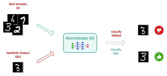
The Discriminator model, on the other hand, takes as input the generated sample as well as the real samples from the domain space with the goal of distinguishing between the two samples (generated versus real).

The following illustration depicts the high-level abstraction of the Discriminator model:

Figure.2

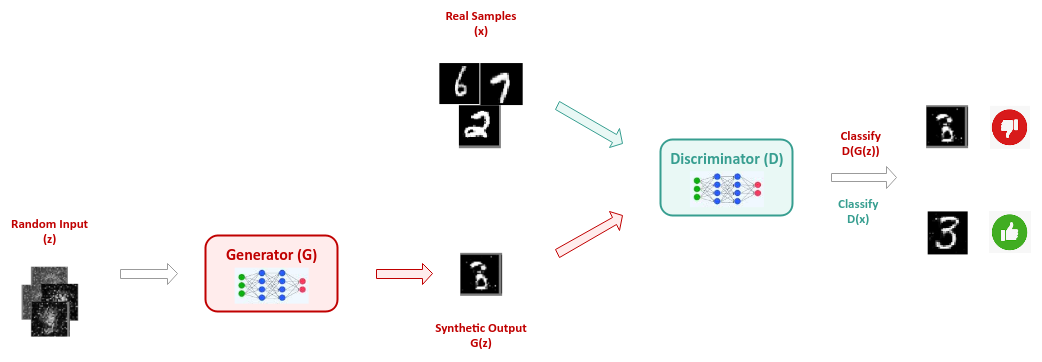
In short, the Generator model and the Discriminator model are engaged in an adversarial cat and mouse game, such that the Generator tries to improve its ability to generate realistic synthetic data samples, while the Discriminator model tries to improve its ability to distinguish between the synthetic samples and the real samples.

The following illustration depicts the high-level abstraction of GAN with both the Generator and the Discriminator models:

Figure.3

Note that the synthetic data samples generated by GAN could apply to any domain such as audio, image, or text. However, GAN models are predominantly used for image generation.

As an example, every image of a person from this site Person Does Not Exist is generated by GAN.

Images are typically generated and classified using the Convolutional Neural Network, and hence it is sometimes referred to as the Deep Convolutional GAN.

Let $G$ represent the Generator model and $D$ the Discrimator model. Also, let represent $z$ the random input generated from the Gaussian (or Normal) distribution $p_z$ and $x$ the real data sample from the distribution $p_{data}$.

According to the GAN Paper, the Generator model $G$ and the Discriminator model $D$ are engaged in a min-max game over their value function $V(G, D)$ which is represented as follows:

$min_G \space max_D \space \space V(G, D) = \mathbb{E}_{x \sim p_{data}}[log(D(x))] + \mathbb{E}_ {z \sim p_z}[log(1 - D(G(z)))]$ $..... \color{red}\textbf{(1)}$

where $\mathbb{E}$ is the expected value and $log$ is the natural logarithm.

In other words, the goal of the Generator model $G$ is to minimize the value function $V(G, D)$, while the objective of the Discriminator model $D$ is to maximize the value function $V(G, D)$.

Let us unpack the above equation $\color{red}\textbf{(1)}$ for a better understanding.

The first part of the above equation $\color{red}\textbf{(1)}$ is the term $\bbox[YellowGreen,2pt]{\mathbb{E}_{x \sim p_{data}} [log(D(x))]}$, which represents the expected value of the Discrimator model $D$ predicting the real data sample $D(x)$ as a real data sample with high confidence.

Note that this term does NOT involve the Generator model $G$. The Discriminator model $D$ wants the value of this term (the expected value or weighted average predictions) to be HIGH.

The second part of the above equation $\color{red}\textbf{(1)}$ is the term $\bbox[Salmon,2pt]{\mathbb{E}_{z \sim p_z}[log (1 - D(G(z)))]}$, which represents the expected value of the Discrimator model $D$ predicting the synthetic data sample $D(G(z))$ as a fake data sample with high confidence.

Note that this term DOES involve the Generator model $G$. The Discriminator model $D$ wants the value of this term (the expected value or weighted average predictions) to be as LOW as possible (predicting it is a fake data sample), while the Generator model $G$ wants the value of this term to be as HIGH as possible (to fool the Discriminator model into believing that the data samples are real).

In short, putting the two terms together, as represented in the above equation $\color{red}\textbf{(1)}$, the Discriminator model $D$ wants to maximize the value of the above equation $\color{red}\textbf{(1)}$, while the Generator model $G$ wants to minimize the value of the above equation $\color{red}\textbf{(1)}$.

Taking a step back, we can observe that the Discriminator model $D$ is nothing more than a Binary Classifier outputting a label of 0 for a fake synthetic data samples and a label of 1 real data samples.

Given that there are two classes (fake or real) for this classification problem, one can use the Binary Cross Entropy (or BCE for short) loss function for training the GAN model.

The BCE loss function is defined as follows:

$L = - \frac{1}{N} \sum (y_i.log(\hat{y_i}) + (1 - y_i).log(1 - \hat{y_i}))$ $..... \color{red} \textbf{(2)}$

where $y$ is the true label (ground truth) and $\hat{y}$ is the predicted label.

For better understanding, let us consider just one data sample and simplify the above equation $\color{red}\textbf{(2)}$ as follows:

$L = y.log(\hat{y}) + (1 - y).log(1 - \hat{y})$ $..... \color{red}\textbf{(3)}$

For real data sample, $y = 1$, $D(x) = \hat{y}$, and the loss function $L$ in equation $\color{red}\textbf{(3)}$ reduces to the following:

$L = log(\hat{y}) = log(D(x))$ $..... \color{red}\textbf{(4)}$

For fake synthetic data sample, $y = 0$, $D(G(z)) = \hat{y}$, and the loss function $L$ in equation $\color{red}\textbf{(3)}$ reduces to the following:

$L = log(1- \hat{y}) = log(1 - D(G(z)))$ $..... \color{red}\textbf{(5)}$

Combining equations $\color{red}\textbf{(4)}$ and $\color{red}\textbf{(5)}$ from above, we get the following:

$L = log(D(x)) + log(1 - D(G(z)))$ $..... \color{red}\textbf{(6)}$

Training is never done on a single data sample, but rather on a batch of data samples. Also, note that the data samples come from a data sample distribution - $p_{data}$ for the real data samples and $p_z$ for the synthetic data samples.

For training over a batch of real data samples, the loss function $L$ in equation $\color{red}\textbf{(4)}$ becomes the average loss and can be represented as follows:

$L = \bbox[YellowGreen,2pt]{\sum p_{data}(x).log(D(x))}$ $..... \color{red}\textbf{(7)}$

Similarly, for training over a batch of random data samples, the loss function $L$ in equation $\color{red}\textbf{(5)}$ becomes the average loss and can be represented as follows:

$L = \bbox[Salmon,2pt]{\sum p_z(z).log(1 - D(G(z)))}$ $..... \color{red}\textbf{(8)}$

Combining equations $\color{red}\textbf{(7)}$ and $\color{red}\textbf{(8)}$ from above, we get the following:

$L = \bbox[YellowGreen,2pt]{\sum p_{data}(x).log(D(x))} + \bbox[Salmon,2pt]{\sum p_z(z).log(1 - D(G(z)))}$ $..... \color{red}\textbf{(9)}$

Notice that the loss function $L$ in equation $\color{red}\textbf{(9)}$ above is similar to the value function $V(G, D)$ in the equation $\color{red}\textbf{(1)}$ way above.

Now, that we have an intuition of how the GAN model works, the training of the GAN model results in the following steps:

Sample a batch of $m$ random data samples from the distribution $p_z$
Sample a batch of $m$ real data samples from the distribution $p_{data}$
Update the model weights of the Discriminator model $\theta_D$ by ascending the stochastic gradient (maximize) the loss function $L$ in equation $\color{red}\textbf{(6)}$ with respect to $D$. That is: $\partial D / \partial \theta_D \: (\frac{1}{m} \sum_{i=1}^{m} [log(D(x_i)) + log(1 - D(G(z_i)))])$
Update the model weights of the Generator model $\theta_G$ by descending the stochastic gradient (minimize) the loss function $L$ in equation $\color{red}\textbf{(6)}$ with respect to $G$. That is: $\partial G / \partial \theta_G \: (\frac{1}{m} \sum_{i=1}^{m} [log(1 - D(G(z_i)))])$. Note the first term becomes $0$ since it does not depend on $G$

Hands-on GAN Using PyTorch

To import the necessary Python module(s), execute the following code snippet:

import torch
import numpy as np
import matplotlib.pyplot as plt
import torchvision.datasets as datasets
import torchvision.transforms as transforms
import torchvision.utils as vutils
from torch import nn
from torch import optim
from torch.utils.data import DataLoader

In order to ensure reproducibility, we need to set the seed to a constant value by executing the following code snippet:

seed_value = 3
torch.manual_seed(seed_value)

To download the MNIST data to the directory ./data, execute the following code snippet:

data_dir = './data'
img_sz = 64
batch_sz = 64

compose = transforms.Compose([
    transforms.Resize(img_sz),
    transforms.ToTensor(),
    transforms.Normalize((0.5,), (0.5,))
])

mnist_dataset = datasets.MNIST(root=data_dir, download=True, train=True, transform=compose)

The above code snippet will ONLY download the MNIST dataset once.

To create an instance of the dataset loader and access the samples in batches, execute the following code snippet:

mnist_loader = DataLoader(dataset=mnist_dataset, batch_size=batch_sz, shuffle=True)

To initialize the variable(s) common to both the Discriminator and Generator models, execute the following code snippet:

# Common to Generator and Discriminator
c_bias = False

To initialize the variables for our Discriminator model hyperparameters, execute the following code snippet:

# For Discriminator - 5 Convolutional Layers
d_leaky_relu_slope = 0.2
d_filter_sz = 64

# Discriminator Layer 1 Convolution
d_l1_in_ch = 1 # Layer 1 Convolution No of channels
d_l1_c_num_k = d_filter_sz # Layer 1 Convolution No of Kernels
d_l1_kernel_sz = 4 # Layer 1 Kernel Size
d_l1_stride = 2 # Layer 1 Convolution Stride
d_l1_padding = 1 # Layer 1 Convolution Padding

# Discriminator Layer 2 Convolution
d_l2_in_ch = d_l1_c_num_k # Layer 2 Convolution No of channels
d_l2_c_num_k = d_filter_sz * 2 # Layer 2 Convolution No of Kernels
d_l2_kernel_sz = 4 # Layer 2 Kernel Size
d_l2_stride = 2 # Layer 2 Convolution Stride
d_l2_padding = 1 # Layer 2 Convolution Padding

# Discriminator Layer 3 Convolution
d_l3_in_ch = d_l2_c_num_k # Layer 3 Convolution No of channels
d_l3_c_num_k = d_filter_sz * 4 # Layer 3 Convolution No of Kernels
d_l3_kernel_sz = 4 # Layer 3 Kernel Size
d_l3_stride = 2 # Layer 3 Convolution Stride
d_l3_padding = 1 # Layer 3 Convolution Padding

# Discriminator Layer 4 Convolution
d_l4_in_ch = d_l3_c_num_k # Layer 4 Convolution No of channels
d_l4_c_num_k = d_filter_sz * 8 # Layer 4 Convolution No of Kernels
d_l4_kernel_sz = 4 # Layer 4 Kernel Size
d_l4_stride = 2 # Layer 4 Convolution Stride
d_l4_padding = 1 # Layer 4 Convolution Padding

# Discriminator Layer 5 Convolution
d_l5_in_ch = d_l4_c_num_k # Layer 5 Convolution No of channels
d_l5_c_num_k = 1 # Layer 5 Convolution No of Kernels
d_l5_kernel_sz = 4 # Layer 5 Kernel Size
d_l5_stride = 1 # Layer 5 Convolution Stride
d_l5_padding = 0 # Layer 5 Convolution Padding

To define our Discriminator model, execute the following code snippet:

class Discriminator(nn.Module):
  def __init__(self):
    super(Discriminator, self).__init__()
    self.layers = nn.Sequential(
      # Layer 1
      nn.Conv2d(in_channels=d_l1_in_ch,
                out_channels=d_l1_c_num_k,
                kernel_size=d_l1_kernel_sz,
                stride=d_l1_stride,
                padding=d_l1_padding,
                bias=c_bias
      ),
      nn.LeakyReLU(d_leaky_relu_slope, inplace=True),
      # Layer 2
      nn.Conv2d(in_channels=d_l2_in_ch,
                out_channels=d_l2_c_num_k,
                kernel_size=d_l2_kernel_sz,
                stride=d_l2_stride,
                padding=d_l2_padding,
                bias=c_bias
      ),
      nn.BatchNorm2d(d_l2_c_num_k),
      nn.LeakyReLU(d_leaky_relu_slope, inplace=True),
      # Layer 3
      nn.Conv2d(in_channels=d_l3_in_ch,
                out_channels=d_l3_c_num_k,
                kernel_size=d_l3_kernel_sz,
                stride=d_l3_stride,
                padding=d_l3_padding,
                bias=c_bias
      ),
      nn.BatchNorm2d(d_l3_c_num_k),
      nn.LeakyReLU(d_leaky_relu_slope, inplace=True),
      # Layer 4
      nn.Conv2d(in_channels=d_l4_in_ch,
                out_channels=d_l4_c_num_k,
                kernel_size=d_l4_kernel_sz,
                stride=d_l4_stride,
                padding=d_l4_padding,
                bias=c_bias
      ),
      nn.BatchNorm2d(d_l4_c_num_k),
      nn.LeakyReLU(d_leaky_relu_slope, inplace=True),
      # Layer 5
      nn.Conv2d(in_channels=d_l5_in_ch,
                out_channels=d_l5_c_num_k,
                kernel_size=d_l5_kernel_sz,
                stride=d_l5_stride,
                padding=d_l5_padding,
                bias=c_bias
      ),
      nn.Sigmoid()
    )

  def forward(self, x):
    x = self.layers(x)
    return x

To initialize the variables for our Generator model hyperparameters, execute the following code snippet:

# For Generator - 5 Convolutional Layers
g_latent_sz = 100
g_filter_sz = 64

# Generator Layer 1 Convolution
g_l1_in_ch = g_latent_sz # Layer 1 Convolution No of channels
g_l1_c_num_k = g_filter_sz * 8 # Layer 1 Convolution No of Kernels
g_l1_kernel_sz = 4 # Layer 1 Kernel Size
g_l1_stride = 1 # Layer 1 Convolution Stride
g_l1_padding = 0 # Layer 1 Convolution Padding

# Generator Layer 2 Convolution
g_l2_in_ch = g_l1_c_num_k # Layer 2 Convolution No of channels
g_l2_c_num_k = g_filter_sz * 4 # Layer 2 Convolution No of Kernels
g_l2_kernel_sz = 4 # Layer 2 Kernel Size
g_l2_stride = 2 # Layer 2 Convolution Stride
g_l2_padding = 1 # Layer 2 Convolution Padding

# Generator Layer 3 Convolution
g_l3_in_ch = g_l2_c_num_k # Layer 3 Convolution No of channels
g_l3_c_num_k = g_filter_sz * 2 # Layer 3 Convolution No of Kernels
g_l3_kernel_sz = 4 # Layer 3 Kernel Size
g_l3_stride = 2 # Layer 3 Convolution Stride
g_l3_padding = 1 # Layer 3 Convolution Padding

# Generator Layer 4 Convolution
g_l4_in_ch = g_l3_c_num_k # Layer 4 Convolution No of channels
g_l4_c_num_k = g_filter_sz # Layer 4 Convolution No of Kernels
g_l4_kernel_sz = 4 # Layer 4 Kernel Size
g_l4_stride = 2 # Layer 4 Convolution Stride
g_l4_padding = 1 # Layer 4 Convolution Padding

# Generator Layer 5 Convolution
g_l5_in_ch = g_l4_c_num_k # Layer 5 Convolution No of channels
g_l5_c_num_k = 1 # Layer 5 Convolution No of Kernels
g_l5_kernel_sz = 4 # Layer 5 Kernel Size
g_l5_stride = 2 # Layer 5 Convolution Stride
g_l5_padding = 1 # Layer 5 Convolution Padding

To define our Generator model, execute the following code snippet:

class Generator(nn.Module):
  def __init__(self):
      super(Generator, self).__init__()
      self.layers = nn.Sequential(
        # Layer 1
        nn.ConvTranspose2d(in_channels=g_l1_in_ch,
                            out_channels=g_l1_c_num_k,
                            kernel_size=g_l1_kernel_sz,
                            stride=g_l1_stride,
                            padding=g_l1_padding,
                            bias=c_bias
        ),
        nn.BatchNorm2d(g_l1_c_num_k),
        nn.ReLU(inplace=True),
        # Layer 2
        nn.ConvTranspose2d(in_channels=g_l2_in_ch,
                            out_channels=g_l2_c_num_k,
                            kernel_size=g_l2_kernel_sz,
                            stride=g_l2_stride,
                            padding=g_l2_padding,
                            bias=c_bias
        ),
        nn.BatchNorm2d(g_l2_c_num_k),
        nn.ReLU(inplace=True),
        # Layer 3
        nn.ConvTranspose2d(in_channels=g_l3_in_ch,
                            out_channels=g_l3_c_num_k,
                            kernel_size=g_l3_kernel_sz,
                            stride=g_l3_stride,
                            padding=g_l3_padding,
                            bias=c_bias
        ),
        nn.BatchNorm2d(g_l3_c_num_k),
        nn.ReLU(inplace=True),
        # Layer 4
        nn.ConvTranspose2d(in_channels=g_l4_in_ch,
                            out_channels=g_l4_c_num_k,
                            kernel_size=g_l4_kernel_sz,
                            stride=g_l4_stride,
                            padding=g_l4_padding,
                            bias=c_bias
        ),
        nn.BatchNorm2d(g_l4_c_num_k),
        nn.ReLU(inplace=True),
        # Layer 5
        nn.ConvTranspose2d(in_channels=g_l5_in_ch,
                            out_channels=g_l5_c_num_k,
                            kernel_size=g_l5_kernel_sz,
                            stride=g_l5_stride,
                            padding=g_l5_padding,
                            bias=c_bias
        ),
        nn.Tanh()
      )

  def forward(self, x):
    x = self.layers(x)
    return x

To initialize variables for the device to train on, the batch size of MNIST data samples, the learning rate, the number of epochs, and the labels for the real and synthetic (fake) data samples, execute the following code snippet:

device = 'cpu'
learning_rate = 0.0002
num_epochs = 3
label_real = 1
label_fake = 0

To define a function to initialize the Discriminator and the Generator model weights, execute the following code snippet:

# Default weights initialized by PyTorch leads to Vanishing Gradient problems.
# Hence, custom weights initialization is required

def custom_weights_init(m):
  classname = m.__class__.__name__
  if classname.find('Conv') != -1:
    m.weight.data.normal_(0.0, 0.02)
  elif classname.find('BatchNorm') != -1:
    m.weight.data.normal_(1.0, 0.02)
    m.bias.data.fill_(0)

To create an instance of the Generator model, execute the following code snippet:

generator = Generator().to(device)
generator.apply(custom_weights_init)

Similarly, to create an instance of the Discriminator model, execute the following code snippet:

discriminator = Discriminator().to(device)
discriminator.apply(custom_weights_init)

To create an instance of the binary cross entropy loss, execute the following code snippet:

criterion = nn.BCELoss()

To create an instance of the optimizer for both the Generator and Discriminator models, execute the following code snippet:

g_optimizer = optim.Adam(generator.parameters(), lr=learning_rate, betas=(0.5, 0.999))
d_optimizer = optim.Adam(discriminator.parameters(), lr=learning_rate, betas=(0.5, 0.999))

To implement the iterative training loop to predict the class, compute the loss, and adjust the model parameters through backward pass, for both the Generator and Discriminator models, execute the following code snippet:

def train_discriminator(data_real, data_fake):
  d_optimizer.zero_grad()

  # Real data
  data_real = data_real.to(device)
  data_real_sz = data_real.size(0)
  x_real_label = torch.full((data_real_sz,), label_real, dtype=torch.float, device=device)
  y_hat_real = discriminator(data_real).view(-1)
  loss_real = criterion(y_hat_real, x_real_label)
  loss_real.backward()

  # Fake data
  z_fake_label = torch.full((data_real_sz,), label_fake, dtype=torch.float, device=device)
  y_hat_fake = discriminator(data_fake).view(-1)
  loss_fake = criterion(y_hat_fake, z_fake_label)
  loss_fake.backward()

  # Update the Discriminator weights
  d_optimizer.step()

  return loss_real + loss_fake

def train_generator(data_fake):
  g_optimizer.zero_grad()
  z_fake_sz = data_fake.size(0)
  z_real_label = torch.full((z_fake_sz,), label_real, dtype=torch.float, device=device)
  y_hat_fake = discriminator(data_fake).view(-1)
  loss_fake = criterion(y_hat_fake, z_real_label)
  loss_fake.backward()
  g_optimizer.step()

  return loss_fake

print('### Starting Training')
for epoch in range(num_epochs):
  print(f'\tEpoch -> {epoch+1}')
  for batch_index, (x_real_0, x_real_1) in enumerate(mnist_loader):
    # Train Discriminator
    x_real = x_real_0.to(device)
    x_real_sz = x_real.size(0)
    z_random = torch.randn(x_real_sz, g_latent_sz, 1, 1, device=device)
    z_fake = generator(z_random)
    d_loss = train_discriminator(x_real, z_fake)

    # Train Generator
    z_fake = generator(z_random)
    g_loss = train_generator(z_fake)

    if batch_index % 50 == 0:
      print(f'\tGAN Model -> Batch: {batch_index}, Generator Loss: {g_loss}, Discriminator Loss: {d_loss}')

The following would be a typical trimmed output:

Output

### Starting Training
	Epoch -> 1
	GAN Model -> Batch: 0, Generator Loss: 2.23104190826416, Discriminator Loss: 1.7122244834899902
	GAN Model -> Batch: 50, Generator Loss: 8.913931846618652, Discriminator Loss: 0.03291315585374832
	GAN Model -> Batch: 100, Generator Loss: 4.616231441497803, Discriminator Loss: 0.17577435076236725
	GAN Model -> Batch: 150, Generator Loss: 7.0666680335998535, Discriminator Loss: 0.0914294421672821
  [... TRIM ...]
	GAN Model -> Batch: 750, Generator Loss: 1.8621577024459839, Discriminator Loss: 0.4158519506454468
	GAN Model -> Batch: 800, Generator Loss: 3.454256534576416, Discriminator Loss: 1.0430299043655396
	GAN Model -> Batch: 850, Generator Loss: 2.7888023853302, Discriminator Loss: 0.20228609442710876
	GAN Model -> Batch: 900, Generator Loss: 4.444871425628662, Discriminator Loss: 0.8754826784133911
	Epoch -> 2
	GAN Model -> Batch: 0, Generator Loss: 7.739803314208984, Discriminator Loss: 1.2408348321914673
	GAN Model -> Batch: 50, Generator Loss: 2.569080352783203, Discriminator Loss: 0.3771322965621948
	GAN Model -> Batch: 100, Generator Loss: 3.3595800399780273, Discriminator Loss: 0.24128982424736023
	GAN Model -> Batch: 150, Generator Loss: 3.3501620292663574, Discriminator Loss: 0.29581916332244873
  [... TRIM ...]
	GAN Model -> Batch: 750, Generator Loss: 3.5940775871276855, Discriminator Loss: 0.24096110463142395
	GAN Model -> Batch: 800, Generator Loss: 3.5626015663146973, Discriminator Loss: 0.13417811691761017
	GAN Model -> Batch: 850, Generator Loss: 0.9706592559814453, Discriminator Loss: 1.0775089263916016
	GAN Model -> Batch: 900, Generator Loss: 1.7001209259033203, Discriminator Loss: 0.6206040978431702
	Epoch -> 3
	GAN Model -> Batch: 0, Generator Loss: 1.8814767599105835, Discriminator Loss: 0.6723608374595642
	GAN Model -> Batch: 50, Generator Loss: 3.032073974609375, Discriminator Loss: 0.17791661620140076
	GAN Model -> Batch: 100, Generator Loss: 4.242057800292969, Discriminator Loss: 0.3889331817626953
	GAN Model -> Batch: 150, Generator Loss: 3.995181083679199, Discriminator Loss: 0.074040487408638
  [... TRIM ...]
	GAN Model -> Batch: 750, Generator Loss: 4.391271591186523, Discriminator Loss: 0.5113582611083984
	GAN Model -> Batch: 800, Generator Loss: 5.010047912597656, Discriminator Loss: 0.24809230864048004
	GAN Model -> Batch: 850, Generator Loss: 4.629855155944824, Discriminator Loss: 0.10992951691150665
	GAN Model -> Batch: 900, Generator Loss: 6.0013227462768555, Discriminator Loss: 0.13961000740528107

Note that this training will take AT LEAST 30 mins to complete !!!

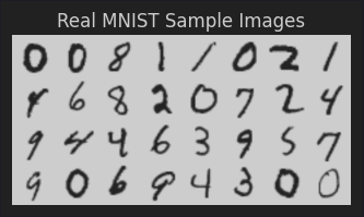
To display some real data samples from the MNIST dataset, execute the following code snippet:

real_batch = next(iter(mnist_loader))
plt.figure(figsize=(4, 4))
plt.axis('off')
plt.title('Real MNIST Sample Images')
plt.imshow(np.transpose(vutils.make_grid(real_batch[0].to(device)[:32], padding=2, normalize=True).cpu(), (1, 2, 0)))
plt.show()

The following illustration depicts real samples images from the MNIST dataset:

Figure.4

To display some synthetic data samples from the Generator model, execute the following code snippet:

with torch.no_grad():
  z_random = torch.randn(img_sz, g_latent_sz, 1, 1, device=device)
  fake_batch = generator(z_random).detach().cpu()
  plt.figure(figsize=(4, 4))
  plt.axis('off')
  plt.title('Synthetic MNIST Sample Images')
  plt.imshow(np.transpose(vutils.make_grid(fake_batch[:32], padding=2, normalize=True).cpu(), (1, 2, 0)))
  plt.show()

The following illustration depicts synthetic samples images produced by the Generator model:

Figure.5

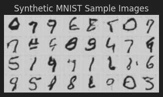
The synthetic image samples generated by the Generator model seem ALMOST close to the real image samples !!!

References

GAN Paper